Linear regression estimates a linear function that maps each input vector to a target variable. In ordinary least squares, the model parameters are estimated by minimizing the sum of squared errors between predicted and observed values. The gradient descent update rule follows directly from this loss function, making linear regression a sensible initial example. For a more thorough review, see (Hastie et al., 2009 Hastie T., et al. (2009). The Elements of Statistical Learning: Data Mining, Inference, and Prediction. Springer. Retrieved from https://books.google.it/books?id=eBSgoAEACAAJ ).
Solution (Python sketch)
The following pseudocode provides a broad idea of the derivations described below. Full code available here.
for _ in range(self.n_iters):
    # Linear model forward pass and calculate MSE.
    y_pred = X.dot(self.w)
    error = y - y_pred
    L = np.mean(error**2) + self.regularization(self.w)
    self.loss_values.append(L)

    # Gradient of mean squared error: dL/dw = -(2/n) X^T (y - y_hat).
    dL_dw = -2 * X.T.dot(error) / X.shape[0] + self.regularization.grad(self.w)

    # Update weights
    self.w -= self.lr * dL_dw
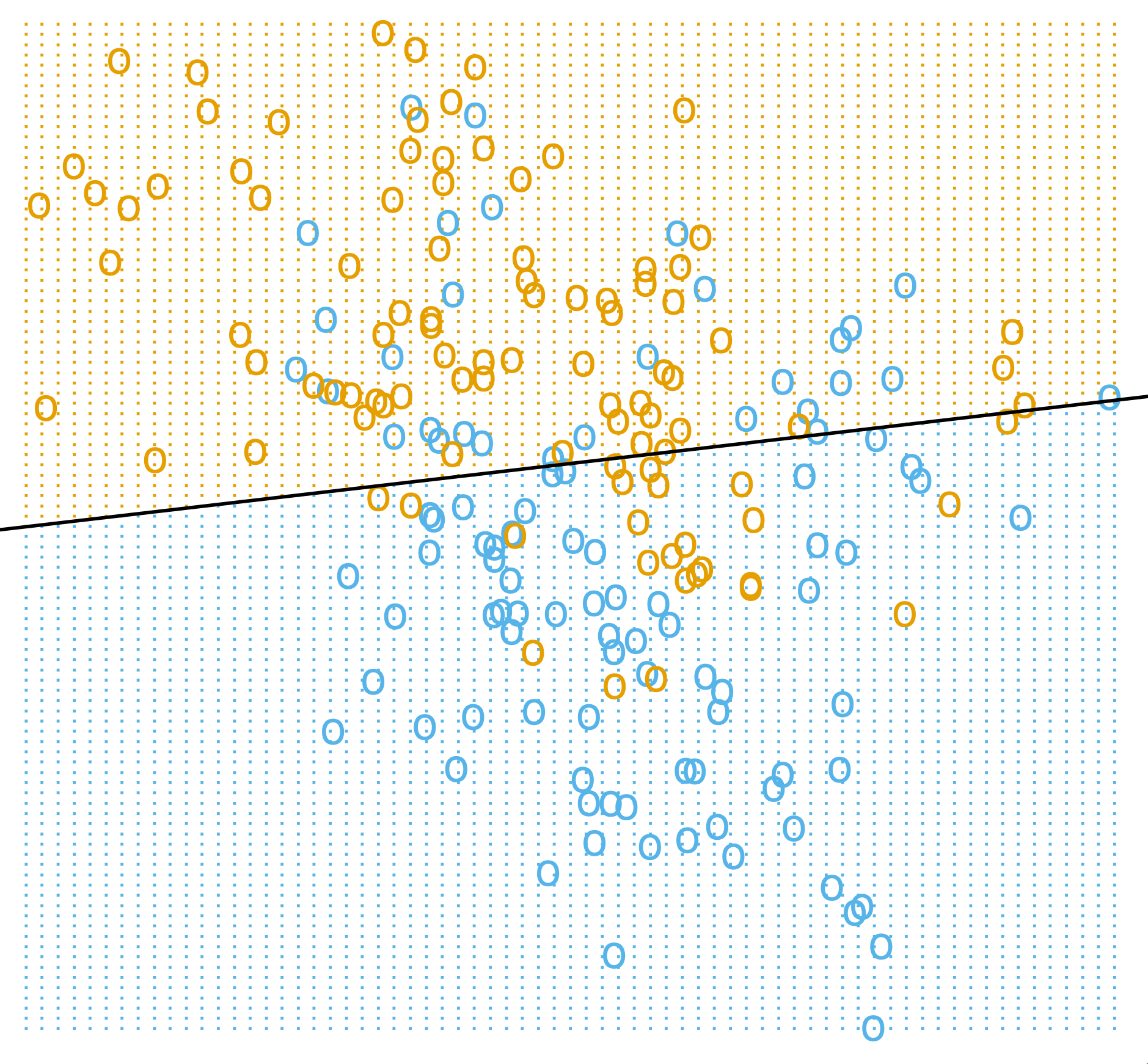
Figure 1: A linear model imposes a single affine decision boundary in the input space. (Image Source: Hastie et al., 2009 Hastie T., et al. (2009). The Elements of Statistical Learning: Data Mining, Inference, and Prediction. Springer. Retrieved from https://books.google.it/books?id=eBSgoAEACAAJ , pp.13)
Setup. Let $X \in \mathbb{R}^{N \times p}$ contain rows $x_i^\top$ and let $y \in \mathbb{R}^N$ contain the targets. If an intercept (bias term) is added, either augment each feature vector with a leading 1 and absorb the bias into $w$, or keep the bias separate. For simplicity, we decide the former approach as it simplifies the code.
Definition 1 (Linear Predictor). For each sample, linear regression predicts by \begin{equation} \hat y_i = x_i^\top w + b. \end{equation}
Definition 2 (Squared Error Objective). Given the sample $(X,y)$, ordinary least squares estimates $\hat w = \arg\min_w L(w)$ (this is the optimization we try to achieve) through the squared-error objective below. \begin{equation} \label{eq:ols-objective} L(w) = \frac{1}{N}\lVert y-Xw \rVert_2^2 = \frac{1}{N}\sum_{i=1}^N (y_i-x_i^\top w)^2. \end{equation} One key term is the residual vector $$ r = Xw-y $$ as it is the main intermediate quantity: it has shape $N$, and both the objective and gradient are built from it.
Derivation. Expanding equation $\eqref{eq:ols-objective}$ gives \begin{equation*} L(w) = \frac{1}{N}(y-Xw)^\top(y-Xw) = \frac{1}{N}\left(y^\top y - 2y^\top Xw + w^\top X^\top Xw\right). \end{equation*} Differentiating equation $\eqref{eq:ols-objective}$ with respect to $w$ gives \begin{equation} \label{eq:ols-gradient} \nabla_w L(w) = -\frac{2}{N}X^\top y + \frac{2}{N}X^\top Xw = \frac{2}{N}X^\top(Xw-y). \end{equation} Note that luckily we have: $X^\top(Xw-y)\in\mathbb{R}^p$, so the gradient matches the parameter vector, which is necessary for compatibility while coding. For a general backpropagation theory beyond linear models, see Deep Learning (Goodfellow et al., 2016 Goodfellow Ian, et al. (2016). Deep Learning. MIT Press. ), pp. 212-213.
Closed Form. Setting the gradient in equation $\eqref{eq:ols-gradient}$ to zero gives the normal equations1 and, when invertible, the closed-form estimator is defined below: \begin{equation} \label{eq:ols-normal} X^\top X \hat w = X^\top y. \end{equation} Because OLS2 minimizes the differentiable quadratic loss in equation $\eqref{eq:ols-objective}$, any minimizer must satisfy $\nabla_w L(w)=0$. If $X^\top X$ is invertible, equation $\eqref{eq:ols-normal}$ gives the closed form solution: \begin{equation} \label{eq:ols-closed-form} \hat w = (X^\top X)^{-1}X^\top y. \end{equation} For coding, the linear system can be solved via QR or SVD, which is faster than explicitly finding the inverse.
Implementation Note
The normal equations (exact solution), QR, SVD, and gradient descent are different ways to compute the estimator. If $X^\top X$ is invertible, the inverse formula, QR and SVD all have the same solution; usually QR or SVD yield faster calculations, but the solution is equally precise.
Regularization is different: once a penalty is added to the loss function, the estimator is no longer the common OLS problem but a modified objective, usually named ridged regression.
Gradient Update. Applying gradient descent to equation $\eqref{eq:ols-objective}$ using equation $\eqref{eq:ols-gradient}$ gives \begin{equation} \label{eq:ols-update} w_{t+1} = w_t - \eta \nabla_w L(w_t) = w_t - \eta \frac{2}{N}X^\top(Xw_t-y). \end{equation} If the bias is kept separate instead of being merged into $X$, the gradients become $$ \nabla_w L = \frac{2}{N}X^\top(\hat y-y), \qquad \frac{\partial L}{\partial b} = \frac{2}{N}\sum_{i=1}^N (\hat y_i-y_i). $$ The bias derivative is just the summed residual because $\hat y_i = x_i^\top w + b$ gives $\partial \hat y_i / \partial b = 1$ for every sample.
Caveats. The algebra above is fairly simple, considering that other problems share similarities in terms of the broad steps that are followed (see the logistic regressor). Nonetheless, this estimator can still be a poor fit for data that is either non-linearly separable or numerically unstable. If columns of $X$ are nearly collinear, $X^\top X$ becomes ill-conditioned and the closed-form solution is unstable. Squared loss also magnifies large residuals, so a small number of outliers can dominate.
If the true conditional mean $\mathbb{E}[Y \mid X = x]$ is nonlinear in $x$, OLS still returns only the best linear approximation in the chosen feature space. In this case, $\mathbb{E}[Y \mid X = x]$ is the true mean of $Y$ conditional on $X = x$; that is, the average outcome obtained by fixing $X = x$ and sampling repeatedly from the population.
Connection. Ridge regression keeps the same setup and gradient, but replaces $X^\top X$ with $X^\top X + \lambda I$. That is the minimal modification when plain ordinary least squares is too unstable.
Citation
If you found this post useful for your work, please consider citing it as:
Razvan Florian Vasile. (March 2026). "Linear Regression". Atom Blog. Retrieved from https://rfvasile.github.io/posts/experiments/linear_regression/.
or
@misc{vasile2026linear-regression-numpy,
    title = "Linear Regression",
    author = "Razvan Florian Vasile",
    note = "Personal blog",
    year = "2026",
    month = "March",
    url = "https://rfvasile.github.io/posts/experiments/linear_regression/"
}
References
- [1] Goodfellow Ian, et al. (2016). Deep Learning. MIT Press.
- [2] Hastie T., et al. (2009). The Elements of Statistical Learning: Data Mining, Inference, and Prediction. Springer. Retrieved from https://books.google.it/books?id=eBSgoAEACAAJ