Logistic regression is used to model a binary label (i.e. 0/1) through a linear function followed by a sigmoid. Broadly speaking, the sigmoid is the common approach for modelling a Bernoulli distribution, which is a statistical model for predicting outcomes involving two distinct categories. Training a model involves maximizing conditional likelihood, or equivalently minimizing binary cross-entropy.
Solution (Python sketch)
The following pseudocode provides a broad idea of the derivations described below. Full code availabe here.
class LogisticRegression(ABC):
    """Base wrapper for the training loop."""

    def _sigmoid(self, logits: Tensor) -> Tensor:
        """Used to obtain probabilities from specified logits"""
        return 1/(1+torch.exp(-logits))

    def fit(self, X: Tensor, y: Tensor) -> LogisticRegression:
        for _ in range(self.n_iters):
            logits = X @ self.weights

            # Apply the sigmoid and the log likelihood function
            p = self._sigmoid(logits)
            p = torch.clamp(p, min=1e-12, max=1-1e-12)
            loss = -torch.mean(y*torch.log(p) + (1-y)*torch.log(1-p))

            # Update step
            step = self.optimizer(X, y)   # N
            self.weights = self.weights - self.lr * step

class GradientDescent(LogisticRegression):
    """Calculate gradient using gradient descent (first order method)."""

    def optimizer(self, X: Tensor, y: Tensor) -> Tensor:
        """Calculate the gradient"""
        logits = X @ self.weights   # (MxN) x (N) -> M
        p = self._sigmoid(logits)   # M
        return torch.mean(X.T * (p-y), dim=1) # (NxM) x (M) -> N x M -> N


class NewtonsMethod(LogisticRegression):
    """Calculate gradient using Newton's method (second order method)."""

    def optimizer(self, X: Tensor, y: Tensor) -> Tensor:
        """Calculate the gradient."""
        z = X @ self.weights    # (MxN) x N -> M
        p = self._sigmoid(z)    # M
        S = torch.diag(p*(1-p)) # MxM

        # Dimensions: (NxM x MxM x MxN)^-1 x NxM x M -> N
        H = X.T @ S @ X
        g = X.T @ (p - y)

        # Apply a dampening term so the system becomes stable
        eps = 1e-4
        I = torch.eye(H.shape[0], dtype=H.dtype, device=H.device)
        step = torch.linalg.solve(H + eps * I, g)
        return step
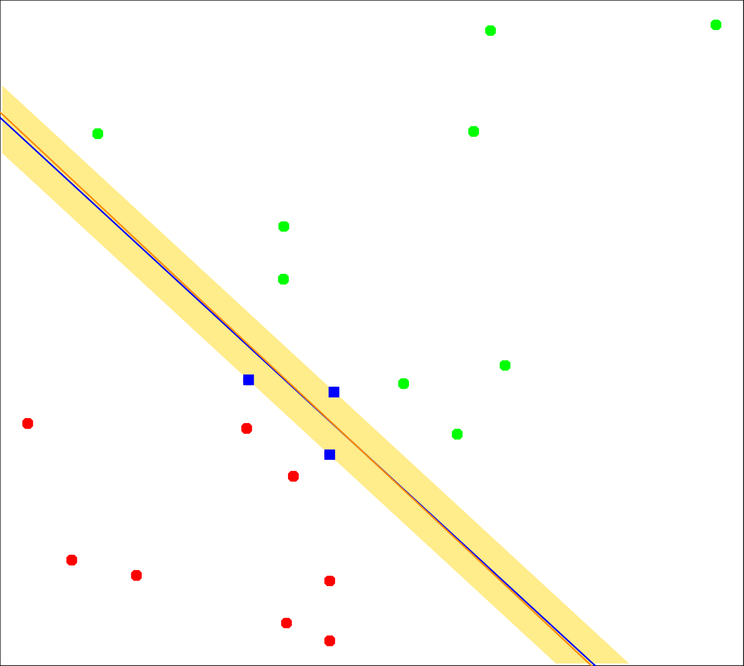
Figure 1: Red and green points denote the two classes. The red line is the decision boundary found by logistic regression. (Image Source: Hastie et al., 2009 Hastie T., et al. (2009). The Elements of Statistical Learning: Data Mining, Inference, and Prediction. Springer. Retrieved from https://books.google.it/books?id=eBSgoAEACAAJ , pp.134)
Model Setup
Setup. Let $X \in \mathbb{R}^{N \times p}$ contain rows $x_i^\top \in \mathbb{R}^{1 \times p}$ and let $y \in \{0,1\}^N$ contain the binary targets. If a bias is used, either augment each feature vector with a leading 1 and absorb the bias into $w$, or keep the bias separate. For coding convenience the former approach is preferred since it streamlines calculations (see here). The explanation below keeps the bias separate.
Definition 1 (Sigmoid). For each sample, logistic regression maps the linear score to a Bernoulli probability. For calculating probabilities we apply the sigmoid function: \begin{equation} \label{eq:logistic-sigmoid} z_i = x_i^\top w + b, \qquad p_i = \sigma(z_i) = \frac{1}{1+e^{-z_i}}. \end{equation} Here $\sigma$ denotes the sigmoid (or logistic) function, which maps the real-valued score $z_i$ to a number in $\{0,1\}$.
The sigmoid derivative is $$ \sigma’(z) = \sigma(z)\bigl(1-\sigma(z)\bigr). $$
To obtain binary outputs, a common approach is to apply thresholding at $0.5$: $$ \hat y_i = \begin{cases} 1, & p_i > 0.5, \\ 0, & \text{otherwise}. \end{cases} $$
Derivation (Sigmoid Derivative)
Start from the sigmoid definition:
$$ p_i = \sigma(z_i) = \frac{1}{1+e^{-z_i}}. $$
Differentiate with respect to $z_i$:
$$ \frac{\partial p_i}{\partial z_i} = \frac{\partial}{\partial z_i}(1+e^{-z_i})^{-1} = -(1+e^{-z_i})^{-2}\frac{\partial}{\partial z_i}(1+e^{-z_i}). $$
Since:
$$ \frac{\partial}{\partial z_i}(1+e^{-z_i}) = -e^{-z_i}, $$
substituting gives:
$$ \frac{\partial p_i}{\partial z_i} = -(1+e^{-z_i})^{-2}(-e^{-z_i}) = \frac{e^{-z_i}}{(1+e^{-z_i})^2}. $$
Now rewrite the result in terms of $p_i$. Because
$$ p_i = \frac{1}{1+e^{-z_i}}, \qquad 1-p_i = 1-\frac{1}{1+e^{-z_i}} = \frac{e^{-z_i}}{1+e^{-z_i}}, $$
we have:
$$ p_i(1-p_i) = \frac{1}{1+e^{-z_i}}\frac{e^{-z_i}}{1+e^{-z_i}} = \frac{e^{-z_i}}{(1+e^{-z_i})^2}. $$
Therefore,
$$ \frac{\partial p_i}{\partial z_i} = p_i(1-p_i). $$
Objective
Definition 2 (Negative Log-Likelihood). Now, to train a model to predict probabilities, logistic regression minimizes the Bernoulli negative log-likelihood: \begin{equation} \label{eq:logistic-objective} L(w,b) = -\frac{1}{N}\ell(w,b) = -\frac{1}{N}\sum_{i=1}^N \left[y_i \log p_i + (1-y_i)\log(1-p_i)\right]. \end{equation} With $z = Xw + b\mathbf 1$ and $p = \sigma(z)$, the same loss is: $$ L(w,b) = -\frac{1}{N}\left(y^\top \log p + (\mathbf 1-y)^\top \log(\mathbf 1-p)\right). $$
Derivation
For one sample: $$ \ell_i = -\left[y_i\log p_i + (1-y_i)\log(1-p_i)\right]. $$ Differentiate with respect to $p_i$: $$ \frac{\partial \ell_i}{\partial p_i} = -\frac{y_i}{p_i} + \frac{1-y_i}{1-p_i} = \frac{p_i-y_i}{p_i(1-p_i)}. $$ Since: $$ \frac{\partial p_i}{\partial z_i} = p_i(1-p_i), $$
the chain rule gives: \begin{equation} \label{eq:logistic-dlogit} \frac{\partial \ell_i}{\partial z_i} = \frac{\partial \ell_i}{\partial p_i}\frac{\partial p_i}{\partial z_i} = p_i-y_i. \end{equation} Here the sigmoid and cross-entropy combine so that the extra factor $p_i(1-p_i)$ cancels.
Result 1 (Stable Per-Sample Form). Implementation-wise, a more stable form is obtained by writing the sample loss as a function of the logit $z_i = x_i^\top w + b$ and the label $y_i$:
For one sample with $p_i = \sigma(z_i)$ and $y_i \in \{0,1\}$, the stable per-sample loss is: \begin{equation*} \ell_i(z_i,y_i) = \log(1+e^{z_i}) - y_i z_i = \operatorname{softplus}(z_i) - y_i z_i. \end{equation*} This form avoids evaluating $\log(\sigma(z_i))$ and $\log(1-\sigma(z_i))$ separately when $|z_i|$ is large.
Derivation
Start from the Bernoulli negative log-likelihood for one sample: $$ \ell_i = -\left[y_i\log p_i + (1-y_i)\log(1-p_i)\right]. $$ Using $$ p_i = \sigma(z_i) = \frac{1}{1+e^{-z_i}} = \frac{e^{z_i}}{1+e^{z_i}}, \qquad 1-p_i = \frac{1}{1+e^{z_i}}, $$ substitute into the loss: $$ \ell_i = -\left[y_i \log\left(\frac{e^{z_i}}{1+e^{z_i}}\right) + (1-y_i)\log\left(\frac{1}{1+e^{z_i}}\right)\right]. $$ Expanding the logarithms gives: $$ \log\left(\frac{e^{z_i}}{1+e^{z_i}}\right) = z_i - \log(1+e^{z_i}), \qquad \log\left(\frac{1}{1+e^{z_i}}\right) = -\log(1+e^{z_i}), $$ so: $$ \ell_i = -\left[y_i\bigl(z_i-\log(1+e^{z_i})\bigr) - (1-y_i)\log(1+e^{z_i})\right]. $$ Collect the two log terms: $$ y_i\log(1+e^{z_i}) + (1-y_i)\log(1+e^{z_i}) = \log(1+e^{z_i}), $$ which yields: $$ \ell_i(z_i,y_i) = \log(1+e^{z_i}) - y_i z_i. $$ Finally, by definition of the softplus function, $$ \operatorname{softplus}(z_i) := \log(1+e^{z_i}), $$ so: $$ \ell_i(z_i,y_i) = \operatorname{softplus}(z_i) - y_i z_i. $$
Optimization
Generally, first-order methods are commonly used for logistic regression. For smaller, more difficult problems, second-order methods such as Newton’s method and IRLS are also common because they can converge in fewer iterations, at the cost of being more compute-expensive.
First-Order Methods
Gradient. Stack the logits into $z \in \mathbb{R}^N$ and the probabilities into $p \in \mathbb{R}^N$. Using equation $\eqref{eq:logistic-dlogit}$ and $z = Xw + b\mathbf 1$, the gradient formulas are: \begin{equation} \label{eq:logistic-gradient} \nabla_w L(w,b) = \frac{1}{N}X^\top(p-y), \qquad \frac{\partial L}{\partial b} = \frac{1}{N}\sum_{i=1}^N (p_i-y_i). \end{equation}
Motivation (Backprop View)
For one sample, it is useful to think of logistic regression as a one-layer model: $$ z_i = x_i^\top w + b, \qquad p_i = \sigma(z_i), \qquad \ell_i = \ell_i(p_i,y_i). $$ Then the chain rule gives: $$ \frac{\partial \ell_i}{\partial w} = \frac{\partial \ell_i}{\partial p_i} \frac{\partial p_i}{\partial z_i} \frac{\partial z_i}{\partial w}. $$ From equation $\eqref{eq:logistic-dlogit}$, $$ \frac{\partial \ell_i}{\partial z_i} = p_i-y_i. $$ Also, $$ \frac{\partial z_i}{\partial w} = x_i, \qquad \frac{\partial z_i}{\partial b} = 1. $$ So for one sample, $$ \frac{\partial \ell_i}{\partial w} = (p_i-y_i)x_i, \qquad \frac{\partial \ell_i}{\partial b} = p_i-y_i. $$ Averaging over all samples gives: $$ \nabla_w L(w,b) = \frac{1}{N}\sum_{i=1}^N (p_i-y_i)x_i = \frac{1}{N}X^\top(p-y), \qquad \frac{\partial L}{\partial b} = \frac{1}{N}\sum_{i=1}^N (p_i-y_i). $$ This is the same chain-rule pattern used in backpropagation; logistic regression is just the single-neuron case with sigmoid output.
Note that $X^\top(p-y) \in \mathbb{R}^p$, so the gradient matches the weights vector. If an $L_2$ penalty $\frac{\lambda}{2N}\lVert w\rVert_2^2$ is added, then $$ \nabla_w L_{\mathrm{reg}}(w,b) = \frac{1}{N}X^\top(p-y) + \frac{\lambda}{N}w, $$ while the bias derivative is commonly left unregularized.
Update Rule. Applying gradient descent to equation $\eqref{eq:logistic-objective}$ using equation $\eqref{eq:logistic-gradient}$ gives: \begin{equation} \label{eq:logistic-update} w_{t+1} = w_t - \eta \frac{1}{N}X^\top(p_t-y), \qquad b_{t+1} = b_t - \eta \frac{1}{N}\sum_{i=1}^N (p_{t,i}-y_i). \end{equation} With $L_2$ regularization, the weight update becomes: $$ w_{t+1} = w_t - \eta \left[\frac{1}{N}X^\top(p_t-y) + \frac{\lambda}{N}w_t\right]. $$
Second-Order Methods
For Newton’s method and IRLS (iteratively reweighted least squares), use the augmented matrix $\tilde X = [\mathbf 1; X]$, the augmented parameter $\tilde w = (b,w)$, and the diagonal matrix $$ S := \operatorname{diag}(p_i(1-p_i)). $$
Hessian. The Hessian of the unregularized loss is: \begin{equation} \label{eq:logistic-hessian} \nabla^2 L(\tilde w) = \frac{1}{N}\tilde X^\top S\tilde X. \end{equation} Because $S$ has nonnegative diagonal entries, equation $\eqref{eq:logistic-hessian}$ is positive semidefinite1, so the objective is convex (so any local minimum is global). This is the matrix used by Newton’s method and IRLS.
Newton Step. Using equation $\eqref{eq:logistic-hessian}$, a Newton step has the form: $$ \tilde w_{t+1} = \tilde w_t - (\tilde X^\top S_t \tilde X)^{-1}\tilde X^\top(p_t-y), $$ which is the basis of IRLS. In difficult problems it often converges in fewer iterations than plain gradient descent, but each step is more expensive because the solution involves solving a linear system.
Implementation notes. Main implementation notes include:
- For stability, the predicted probabilities are clamped to $[10^{-12}, 1-10^{-12}]$ before taking logarithms.
- In Newton’s method, a damping term term is used, replacing $H$ with $H+\varepsilon I$ for $\varepsilon=10^{-4}$, to stabilize the linear solver when the Hessian is ill-conditioned (i.e. when the columns are nearly linearly dependent).
- Experiments confirm that Newton’s method converged faster and used $\eta=1.0$, while gradient descent still required a relatively large learning rate, $\eta=0.1$.
A symmetric matrix $A$ is positive semidefinite if $v^\top A v \ge 0$ for every vector $v$, so its quadratic form is never negative. ↩︎
Citation
If you found this post useful for your work, please consider citing it as:
Razvan Florian Vasile. (March 2026). "Logistic Regression". Atom Blog. Retrieved from https://rfvasile.github.io/posts/experiments/logistic_regression/.
or
@misc{vasile2026logistic-regression-numpy,
    title = "Logistic Regression",
    author = "Razvan Florian Vasile",
    note = "Personal blog",
    year = "2026",
    month = "March",
    url = "https://rfvasile.github.io/posts/experiments/logistic_regression/"
}
References
- [1] Hastie T., et al. (2009). The Elements of Statistical Learning: Data Mining, Inference, and Prediction. Springer. Retrieved from https://books.google.it/books?id=eBSgoAEACAAJ